You don’t have to create complicated formulas to combine text from multiple columns to a single column. In this Excel tip, we will show you how to quickly and easily combine your data from multiple columns into one column.
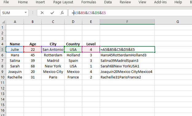
In the example below. We have five different columns of data and we need this data to be combined into one column. We use the "&" sign to achieve this.
Download the workbook to practice.
- First, put your cursor into the cell in which you want the combined value, in our example we used F5.
- Next, put your cursor into the Formula Bar and type the equals sign, “=”
- Then, select the first cell you want to include which is A5 for this example, then type an ampersand sign “&” into the formula.
- Then, select the second cell you want to include, in our example it is B5 and follow it with an ampersand sign “&” as well. Repeat this process for all the columns that you would like combined.
For this example, the formula is: =A5&B5&C5&D5&E5
- Then, select the ‘enter’ key and your combination will be visible.
- Finally, keeping the cell selected, you should see your formula and you can hover over the small dot on the bottom right of the cell. This is the Fill. Click and drag the dot downward so that the formula is copied to the remaining rows. Or, since the column prior includes values you could simply double-click on the dot and your formula will automatically fill in all the rows.

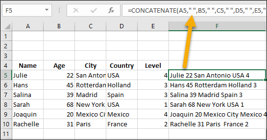
If you would like spaces between text, you will need to use the Concatenate formula.
- To add space between words, simply add quotation marks around a space as well as comma separators. Don’t forget the comma separators!
Your formula will be: =CONCATENATE(A5,” “,B5,” “,C5,” “,D5,” “,E5,”)

