In a previous tip, we explained how you can easily remove duplicate rows from your data using the Remove Duplicates function.   You can find it here.   At times though, you may just want to highlight duplicate rows without actually deleting them.   In this tip, we show you how you can do this using an Excel formula. 1. First, you need to make sure that your data is sorted. Assuming it starts in cell A1 and has headings, select cell A2 and then click Sort A to Z on the Data tab on the menu ribbon.
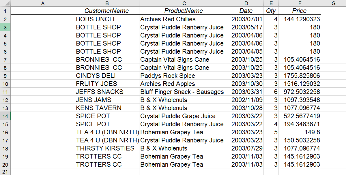
2. Next, enter a new column in front of column A by right clicking on the label for column A and selecting Insert.
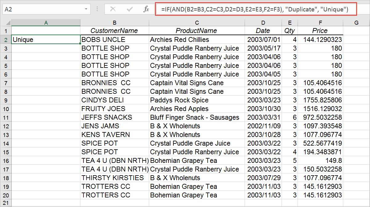
3. Now, in cell A2, we're going to make use of an IF and AND function to identify duplicates. Enter the following: =IF(AND(B2=B3,C2=C3,D2=D3,E2=E3,F2=F3), "Duplicate", "Unique") Note that the formula is checking to see whether the value in cell B2 is equal to the value in cell B3 and whether the value in cell C2 is equal to the value in cell C3 and whether the value in cell D2 is equal to the value in cell D3, etc.   If all combinations are equal, then it implies that the row is a duplicate and the function returns the text "Duplicate".   If not, then "Unique" is returned.
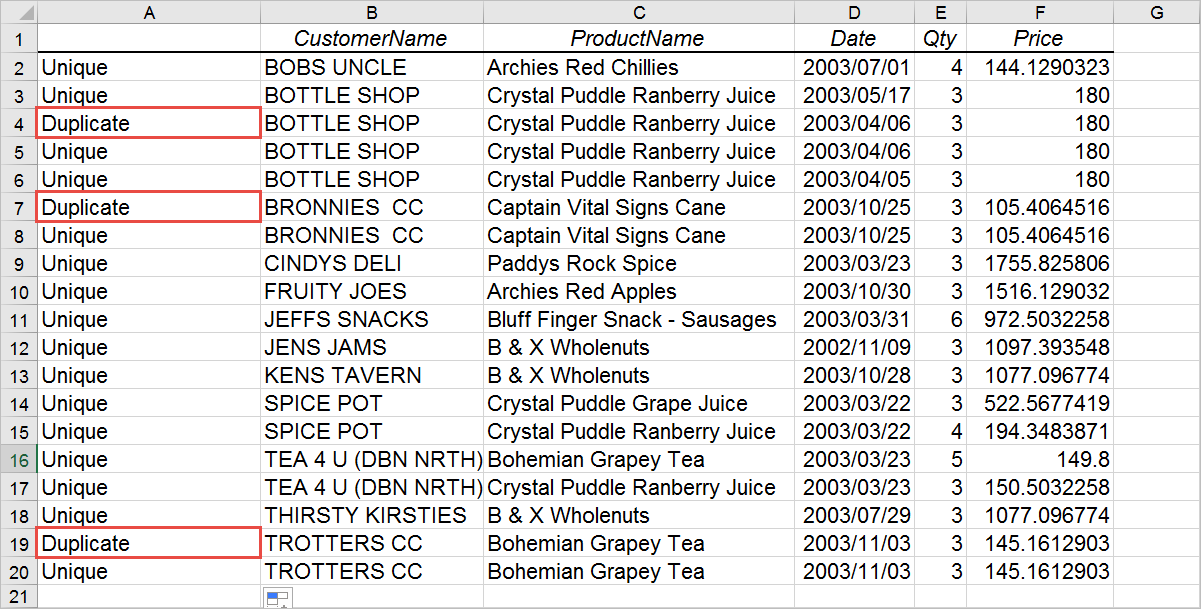
Also keep in mind that your data will likely vary in the number of columns it has and you will need to do the cell comparison for each column that you have.   Furthermore, you may regard a duplicate as consisting of a subset of columns.   For example, in the above data, I might think of a row as being duplicated only if the Customer Name and Product Name are the same.   In that case you would only do the cell comparison for those rows. 4. Now, all you need to do is use the Excel fill handle and copy the formula down to the rows below it. You will notice that any duplicates are identified.
Through the power of Excel functions, you can easily identify duplicate rows which can make working with your data more efficient.